My last boggle post presented an exciting insight that yielded a 30x speedup. This meant two things:

1. I could find the globally-optimal 3x4 Boggle board in ~19 hours using three cores on my laptop, rather than 8-9 hours on a 192-core cloud instance.
2. My cost estimate for finding the globally-optimal 4x4 Boggle board dropped from $500,000→$15,000.

That was still more than I was willing to pay, but it brought me within a factor of 10 of the ultimate goal.

I was able to find another ~10x of optimizations, and I was able to find the best 4x4 board (more on this soon!). What got me there wasn’t an exciting insight. Instead, it was a series of incremental wins that stacked together nicely. This post presents four of them:

• Orderly Bound
• Lift → Orderly Force / Merge
• Inline Child Nodes and Arenas
• Variable-depth Switching

Orderly Bound

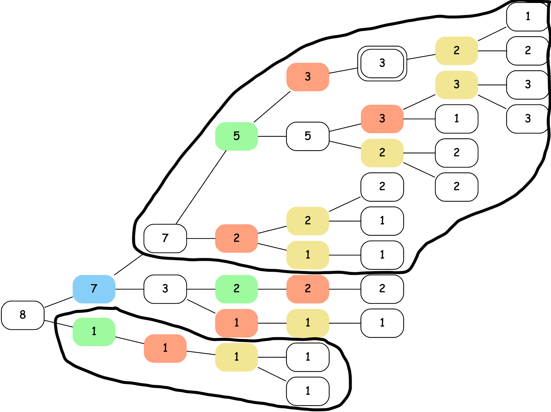
The last post presented Orderly Trees. Here’s what one looked like for a 2x2 board class:

This represents the board class ab cd ef gh, which contains sixteen possible Boggle boards. The blue node is ab, the green nodes are cd, the orange nodes are ef and the yellow nodes are gh.

To calculate the upper bound for a particular board, you take the branches corresponding to its letters and sum them up. Here’s adeg, for example:

To get the Multiboggle score, you add up all the points on the dark, parenthesized cells. So 3 + 2 + 2 + 1 = 8, which is the correct bound.

In practice, we usually want to partially evaluate boards. So we first try making a choice between “A” and “B” for the first cell, and use the tree to calculate an upper bound for both a cd ef gh and b cd ef gh. If either of these has a bound less than our best known score, we’re done. If not, we need to split the next cell: a c ef gh and a d ef gh, etc.

Previously, I calculated these bounds by traversing the tree independently for each set of forced cells. This has low memory cost, but it does lots of duplicated work. There are many identical calculations in the bounds for ab cd ef gh and a cd ef gh, for example.

The new “orderly bound” algorithm does this more efficiently by taking advantage of the “orderly” structure of the tree. The idea is to maintain stacks of pointers, organized by cell. So there’s one stack of blue pointers, one stack of green pointers, etc. To force the blue cell to be a, you pop it off the stack (there’s only one blue cell) and push the next green and orange choice cells you see onto their stacks. You can keep track of the bound on the board class as you do this, which lets you bail out as early as possible.

Here’s an animation of how that looks for boards in ab cd ef gh with a bound > 7:

The active nodes in the stacks have a * next to them. Sum nodes with parentheses indicate where the algorithm is advancing. This is kind of like a DFS.

This was something like a 10x speedup over the previous system, which translated into an overall 2-3x speedup on 3x4 board classes. I’d initially hoped that this system would let me get rid of the lifting operation entirely, but that didn’t pan out. The best approach was to lift a few times and then run OrderlyBound. Hybrid always wins.

This puzzled me for a while because I mistakenly thought that OrderlyBound was linear. But I eventually realized that, while it only visits each node once in this 2x2 example, it has pretty heinous backtracking behavior for larger boards. Lifting helps to mitigate that.

Lift → Orderly Force / Merge

The sequence for upper-bounding a class of Boggle boards is:

1. Build an Orderly Tree for that board class.
2. Do a few lift operations to synchronize choices across subtrees.
3. Call OrderlyBound.

Creating an “Orderly Bound” that was tailor-made for orderly trees was a big win. So what about a tailor-made lift operation?

While I was able to implement something like this, the bigger win came from reevaluating the decisions that had led me to use the “lift” operation in the first place. Recall from my earlier post that “lifting” pivots a single choice node all the way to the top of the tree.

But if you have two choices for a cell (say a and b), then an alternative is to produce two trees, one with that cell set to a and another with that cell set to b. I call this a “force” operation. In the past, I preferred “lift” to “force” because it let me compress and deduplicate subtrees.

When I switched to orderly trees, however, compression and deduplication stopped being helpful. So I threw them out and switched from “lift” back to “force.” Dropping the fields required required for deduplication was a huge RAM savings.

For an orderly tree, forcing a cell winds up being mostly a “merge” operation on subtrees. For example, to force the first cell (blue) to be a, we merge the top subtree, which corresponds to a, and the lower subtree that starts with a green cell, which corresponds to words that don’t use the first cell (namely ”GED”, which is apparently a type of fish).

This merge operation winds up being quite efficient to implement using iterators that advance in lockstep.

Inline Child Nodes and Arenas

Unlike the other optimizations, this one has nothing to do with Boggle. It’s pure C/C++!

The first time I ran my Boggle solver in the cloud, I was surprised by how much memory I used and by how much faster my code ran on my M2 Macbook than in the cloud. One theory was that Apple’s chips have very high memory bandwidth, and this might be a bottleneck for me on the Intel CPUs in the cloud. So I wanted to reduce my memory usage.

The vast majority of memory in the Boggle solver is used to store a tree structure. After removing unnecessary properties from my EvalNode class, it looked like this:

class EvalNode {
  int8_t letter_;
  int8_t cell_;
  uint16_t points_;
  uint32_t bound_;
  vector<EvalNode*> children_;
}

sizeof(EvalNode) is 32 bytes for this structure on a 64-bit system. I allocate hundreds of millions of these, so saving even a few bytes makes a big difference.

The vast majority of the space is used by the children_ vector. Here’s what the memory layout looks like:

The small fields are organized efficiently into eight bytes. But then the vector takes up the remaining 24 bytes. So how is std::vector implemented? It usually looks something like this:

template <class T>
class vector {
  T* data_;         // points to first element
  T* end_;          // points to one past last element
  T* end_capacity_; // points to one past internal storage
};

I’d always assumed it stored a count, but this three pointer system is clever. It makes it very fast to check whether you’re at the end of a vector, and it frees the implementation from having to care about how big a pointer is.

For us, the gist is that we always store three pointers (24 bytes) directly in the EvalNode structure and then store the child pointers themselves in some other array. In practice most nodes have zero, one or two children. So this winds up being inefficient in a few ways:

1. The three pointers use a lot of space compared to the typical number of child pointers.
2. Because the vector allocates lots of small backing arrays, memory may be fragmented and there’s lots of overhead in managing it.
3. Accessing a child requires going through two pointers.

There’s a classic trick for improving this situation. Instead of using vector<T> children , use T* children[] to store an indeterminate number of child pointers directly in the struct:

class EvalNode {
  int8_t letter_;
  int8_t cell_;
  uint16_t points_;
  uint8_t num_children_;  // new
  uint8_t capacity_;      // new
  uint32_t bound_;
  EvalNode* children_[];  // indeterminate array
}

Now the memory layout looks like this:

sizeof(EvalNode) evaluates to 16 bytes now, but it’s really 16+8*capacity. If you want a node with two children, you allocate 32 bytes and use placement new.

This has some pros and cons. First, the pros:

• The structure is smaller. For a zero-child EvalNode, it’s half the bytes. It can store up to two children and still remain smaller than the old structure, not even including the side buffer.
• It doesn’t allocate memory in an outside array. All the memory is in the structure itself. This reduces fragmentation and means that accessing a child only requires chasing a single pointer.

The cons:

• We have to store the number of children and the capacity of the node. These only take one byte each (nodes have a maximum of 16 children), but this is enough to screw up the alignment of the structure. Six of the sixteen bytes are unused! This is inefficient, but unavoidable without bitpacking.
• It’s hard to add capacity to a node. This is also an issue with vectors, but that complexity is hidden from us. To add a child to a node that’s “at capacity,” we have to allocate a new, larger node and copy everything over.

When I implemented this, the pros vastly outweighed the cons. For 4x4 boards, this reduced memory usage by 20-30% and gave me something like a 40% speedup. A big part of this was that I was able to make more effective use of an arena for memory management. With the new structure, destroying a tree just required deallocating a few large buffers. Previously, it required deallocating millions of little backing arrays for children_.

This improved memory use and management made the final optimization possible.

There were two other things I learned from this optimization that I wanted to note:

1. Long ago, I’d learned to use this trick by putting T* child_[0] as the last property of a struct. This [0] form was never standard and has been obsolete since C99. It’s more correct to write T* child_[]. And as of C++11, this saves you from a footgun: for (auto child : child_) is valid (but not what you want) with child_[0] but is a compile error with child_[].
2. C and C++ compilers are not allowed to reorder properties in a class. So it can pay off to think carefully about alignment and the size of each field.

Update: I later split EvalNode into SumNode and ChoiceNode classes, which let me get both of them down to 8 bytes with no waste.

Variable-depth Switching

To prove that a class of Boggle boards doesn’t contain any individual boards with more than N points, the procedure is:

1. Build an orderly tree for that class.
2. Recursively call Orderly Force some number of times to produce lots of subtrees.
3. Call Orderly Bound on each of those subtrees to get candidate boards with high Multiboggle scores.
4. Run those candidate boards through a plain old Boggle solver to check their true Boggle score.

The depth at which you switch from Force to Bound is a key choice. It’s ultimately a memory/speed tradeoff. More forcing reduces the exponential backtracking behavior of the Orderly Bound algorithm, but requires more RAM.

Previously, I’d used a fixed depth as the switchover point. I couldn’t set it any higher than depth=4 without running into memory problems. But for really hard 4x4 board classes, I found that higher depths were better.

After all the memory optimizations and the switch from Lift to Force, it became practical to use a variable depth. For harder subtrees, I could force more cells before switching over OrderlyBound. I used the upper bound on the current subtree as a proxy. If it got within a factor of 2.5x of the best known board, I’d switch over to OrderlyBound.

This didn’t have much of an effect on 3x4 boards, but it was something like a 2-3x speedup for the hardest 4x4 boards without too much of a RAM penalty. In practice, this sometimes used a lot of forces, up to 12. It would have forced all the cells if I let it, but this tended to use too much RAM.

Conclusion

The lesson here is that when you come up with an exciting new idea, it might force you to reevaluate other decisions that you’ve made. If A was faster than B with the old system, B might be faster than A in the new one.

All these optimizations added up to at least a 10x speedup on my laptop. And given the reduced RAM usage, I was hopeful that these improvements would be at least as big on the Intel CPUs in the cloud.

A $1,500 cloud run is much more palatable than a $15,000 cloud run. But more on that in the next post!