Here’s a map of Arizona’s eight congressional districts as determined by their statehouse (left) and the algorithm (right):

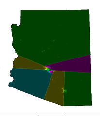
Check out Arizona’s second congressional district!
The splitline algorithm is quite simple. You find the shortest line which splits the state’s population in half. Then find the shortest splitlines in those halves, until you have enough districts. The exact details are here.
I like the simplicity of this approach, but I think there’s some benefit to having coherent districts, i.e. a community having their own representative instead of being split between two representatives of other communities. That being said, I don’t see much evidence that legislatures do this right now, and it seems like a hard thing to incorporate into an algorithm. The splitline approach certainly seems better than the status quo!
I also enjoyed their discussion of Range Voting, a generalization of Approval Voting (Approval Voting is a system in which you say whether you’re OK with each candidate, rather than picking a single one).
In Range Voting, you give each candidate a rating from 0-10, or maybe 0-100. The candidate with the highest average rating wins. By letting you consider each candidate independently (instead of choosing just one or ranking them), it avoids some of the pitfalls inherent in preferential voting systems. And it has more appeal than Approval Voting because it’s more expressive: I can say that I like candidate A more than candidate B (who I’m just OK with), rather than just saying that I approve of both. Even mother nature likes range voting: Honeybees have evolved a form of it!
One interesting thought: if a state switched to using range voting or instant runoff voting, how would it affect the National Popular Vote Bill? Can we have both?
]]>Under the U.S. Constitution, the states have exclusive and plenary (complete) power to allocate their electoral votes, and may change their state laws concerning the awarding of their electoral votes at any time. Under the National Popular Vote bill, all of the state’s electoral votes would be awarded to the presidential candidate who receives the most popular votes in all 50 states and the District of Columbia. The bill would take effect only when enacted, in identical form, by states possessing a majority of the electoral votes—that is, enough electoral votes to elect a President (270 of 538).
Intuitively, you’d expect this bill to be popular in states with:
- Large populations
- Very predictable voting patterns
These are the states like California and Texas which are large, but completely neglected under the current presidential voting system. Putting on our Nate Silver hat, we can try to quantify this. A state is large if it has lots of Electoral Votes. A state has predictable voting patterns if it differed considerably from the national popular vote in the last election. A state should support the NPV bill if it ranks highly in both of these senses:
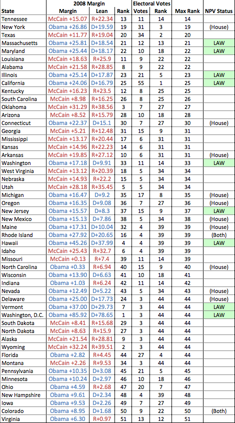
For example, California ranks #1 in Electoral Votes (it has 55). It voted for Obama by a margin of 24% in 2008. The nation as a whole voted for Obama by a margin of 7%, so we say that California leans Democratic by 17%. Amongst all states, this is the 25th largest lean. California’s score is the larger of these two numbers (25). Repeat this analysis for all 50 states and the District of Columbia and you’ll get the chart above.
It’s not surprising to see California, Texas and New York near the top of the list. These are the three largest states, but they do not factor into presidential elections at all. Tennessee surprised me at the top of the list, but with 11 EVs and a 20+ point Republican lean, it would clearly benefit from a change in the system.
If the top three states in this list (Tennessee, Texas, New York) all passed the NPV bill, it would have 210 of the 270 EVs it needs to go into effect. Were that to happen, I believe we’d start to hear a lot more about it in the media.
Raw data here (Excel format). For what it’s worth, I now understand why Nate uses images for the tables on his blog: getting a formatted table out of Excel in any other format is nearly impossible!
]]>For those not familiar with the basic story (I wasn’t before I moved to SF), City Supervisor Dan White quit his job, then asked to be reinstated. When Mayor George Moscone refused, White returned to city hall with a gun and murdered Moscone and Supervisor Harvey Milk, who happened also be the first openly-gay elected official in the country. Another Supervisor, now-Senator Dianne Feinstein became mayor as a result of these killings.
An NPR show yesterday included a clip of Feinstein giving a dramatic press conference announcing the deaths. Much to my surprise, an original copy of that night’s newcast has found its way online.
The Feinstein press conference is at 2:10. Listen to the gasps. The 70′s production is jarring to look at now though, except for the cars, the shots of San Francisco could have been taken yesterday.
I couldn’t figure out whether this is an isolated clip or part of a larger collection. How cool would it be if all of NBC’s old newscasts were online?
]]>Not to suggest that presidents have any impact on the stock market…
| President | End Date | Close | Change | % Change | Annual |
|---|---|---|---|---|---|
| G.W. Bush | 14-Nov-08 | $873.29 | -$469.25 | -34.95% | -5.35% |
| Clinton | 20-Jan-01 | $1342.54 | $909.17 | 209.79% | 15.18% |
| G.H.W. Bush | 20-Jan-93 | $433.37 | $146.74 | 51.19% | 10.89% |
| Reagan | 20-Jan-89 | $286.63 | $154.98 | 117.72% | 10.21% |
| Carter | 20-Jan-81 | $131.65 | $28.68 | 27.85% | 6.34% |
| Ford | 20-Jan-77 | $102.97 | $22.11 | 27.34% | 10.37% |
| Nixon | 9-Aug-74 | $80.86 | -$20.83 | -20.48% | -4.05% |
| Johnson | 20-Jan-69 | $101.69 | $32.08 | 46.09% | 7.62% |
| JFK | 22-Nov-63 | $69.61 | $9.65 | 16.09% | 5.40% |
| Eisenhower | 20-Jan-61 | $59.96 | $33.82 | 129.38% | 10.94% |
I thought that, for each simulation of the election, Nate sorted the states by margin of victory for the overall winner. Then he’d start adding up electoral votes. The state that tipped the winner over 270 would be the “tipping point state” for that simulation.
While writing this blog post, I discovered that I had completely misunderstood this list! Nate describes the actual calculation of his list in this post. It’s quite involved, but better captures the intuition of a “tipping point state”.
Just for fun, I figured out what the 2008 Election’s tipping point state was using the methodology I’d originally thought Nate did. And it was… Colorado! Obama took Colorado with 54.40% of the vote, the 23rd most lopsided total. It takes him from 262 to 271 Electoral Votes.
Full list of states, margins of victory and electoral votes below the fold.
| State | % Obama | Total EV |
|---|---|---|
| D.C. | 93.42% | 3 |
| Hawaii | 72.93% | 7 |
| Vermont | 67.89% | 10 |
| Rhode Island | 64.13% | 14 |
| Massachusetts | 63.13% | 26 |
| New York | 62.87% | 57 |
| Illinois | 62.37% | 78 |
| Maryland | 62.22% | 88 |
| California | 62.21% | 143 |
| Delaware | 61.99% | 146 |
| Washington | 58.84% | 157 |
| Maine | 58.73% | 161 |
| Michigan | 58.38% | 178 |
| New Mexico | 57.61% | 183 |
| New Jersey | 57.37% | 198 |
| Wisconsin | 57.04% | 208 |
| Oregon | 56.66% | 215 |
| Nevada | 56.35% | 220 |
| Pennsylvania | 55.24% | 241 |
| Minnesota | 55.22% | 251 |
| New Hampshire | 54.82% | 255 |
| Iowa | 54.70% | 262 |
| Colorado | 54.40% | 271 |
| Connecticut | 53.44% | 278 |
| Virginia | 52.26% | 291 |
| Ohio | 51.98% | 311 |
| Florida | 51.27% | 338 |
| Indiana | 50.48% | 349 |
| Nebraska 2nd | 50.24% | 350 |
| North Carolina | 50.17% | 365 |
| Missouri | 49.90% | 376 |
| Montana | 48.24% | 379 |
| Georgia | 47.25% | 394 |
| South Dakota | 45.70% | 397 |
| Arizona | 45.64% | 407 |
| North Dakota | 45.57% | 410 |
| South Carolina | 45.47% | 418 |
| Nebraska 1st | 44.80% | 419 |
| Texas | 44.08% | 453 |
| West Virginia | 43.33% | 458 |
| Mississippi | 43.07% | 464 |
| Kentucky | 42.37% | 472 |
| Tennessee | 42.36% | 483 |
| Kansas | 42.17% | 489 |
| Nebraska | 41.83% | 491 |
| Louisiana | 40.50% | 500 |
| Arkansas | 39.78% | 506 |
| Alabama | 39.10% | 515 |
| Alaska | 37.08% | 518 |
| Idaho | 36.86% | 522 |
| Utah | 35.20% | 527 |
| Oklahoma | 34.36% | 534 |
| Wyoming | 33.38% | 537 |
| Nebraska 3rd | 30.06% | 538 |
The first half of the show, which covers McCain and Obama’s early lives, is the more interesting, or at least less familiar. Frontline did a great job of digging up old videos. There’s a recording of McCain in the POW camp. There’s a recording of Obama giving a speech at Harvard Law in 1990. He looks different, but the cadence of his speech is eerily familiar. It’s also interesting to see speeches that McCain gave in the past. He’s noticeably more relaxed than he has been in the debates. A particular standout is his exchange with John Stewart in 2006.
My main problem with the episode was its lack of depth. This was more of a problem with the latter half, where I could see the gaps in their coverage of stories with which I was already familiar. The biggest questions they asked but left unresolved related to Reverend Wright. They said it was shocking that the Clinton campaign didn’t use him against Obama until after Super Tuesday, but never offered an explanation of why. I’ve often wondered this as well. If the Reverend Wright controversy had struck before Obama was ahead in delegates, Hillary might well be the nominee.
]]>McCain (R) 46%
Obama (D) 50%
Margin of Error: +/-3.7%
Tables like this appear on TV and in newspapers all the time. But they’re never accompanied by any explanation of how to interpret the margin of error. Commentators usually interpret it in one of two ways:
- Obama is ahead by more than the margin of error, hence his lead is statistically significant.
- That “+/-” means either number could be off by that amount. If you added 3.7% to McCain’s 46% and subtracted 3.7% from Obama’s 50%, McCain would actually be ahead. So Obama’s lead is not statistically significant; it is less than twice the margin of error.
In either case, they are wrong.
So what’s the right way to interpret the margin of error? A lead is significant if it is 1.6 times the margin of error or greater. That’s 5.9% for our poll, so Obama’s lead is not significant.
This is a strange, non-intuitive rule, which explains why commentators don’t use it. The derivation is more revealing than the rule itself.
Obama’s lead is “statistically significant” if there’s a 95% probability that Obama is actually ahead. The “95%” is completely arbitrary, but the probability
P(Obama ahead)
is quite interesting. I wish news organizations would report this probability instead of the margin of error. It’s easier to interpret the statement “There’s an 86.5% chance that Obama is ahead” than a statement about margins of error.
These margins of error, incidentally, are just one over the square root of the sample size. For the poll described above, there were 732 voters surveyed. The square root of 732 is 27 and one over that is .03696 or 3.7%. The reported margin of error is not a standard deviation.
The probability that Obama is ahead can be determined using Bayes' Rule, which quantifies the effect of evidence on our belief in a hypothesis. It relates a Hypothesis (H) and an Observation (O):
H = Obama is ahead of McCain.
O = In a poll of 732 likely voters, 50% preferred Obama and 46% preferred McCain.
Here it is:
Bayes’ Rule: P(H|O) = P(O|H)/P(O) * P(H)
This rule is important enough that each of these quantities has a name:
- P(H) is the prior probability, our belief that the hypothesis is true before seeing additional evidence.
- P(O|H) is the likelihood function, the probability of seeing the evidence if the hypothesis were true.
- P(O) is the marginal probablity, the probablity of seeing the evidence at all. It’s often thought of as a normalizing term.
- P(H|O) is the posterior probability. It’s what we’re really after, the likelihood of the hypothesis in light of new evidence.
Let’s start with the likelihood function, P(O|H). What are the odds of seeing this survey is a certain portion p of voters prefer Obama? It follows from the binomial formula:
pO = portion of voters preferring Obama
pM = portion of voters preferring McCain
a = pO * N (number of voters who prefer Obama)
b = pM * N (number of voters who prefer McCain)
N = a + b (total decided voters)
P(O|H) = B(a, b) = N! / (a! b!) * pO^a (1-pO)^b
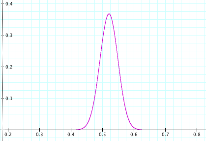
This is a binomial distribution over pO. Notice that we’re only considering the two-way vote here, the 96% of the electorate that prefers either McCain or Obama.
To aid in the application of Bayes’ Rule, statisticians have developed the notion of a conjugate prior. The conjugate prior for the binomial distribution is the beta distribution. This means that, if our likelihood function is a binomial distribution, we can choose a beta distribution for our prior probability and get another beta distribution for the posterior probability.
In this case, it’s simplest to assume a uniform distribution for Obama’s portion of the vote. In other words, it’s equally probable that he’ll get 1% of the vote as it is that he’ll get 50% or 99% of it. Mathematically, if pO is the portion of voters who prefer Obama, then
pO ~ U(0, 1) = B(1, 1)
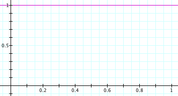
Bayes’ rule then gives the following distribution for pO after observing the poll:
pO’ ~ B(a + 1, b + 1) = B(pO * N + 1, pM * N + 1)
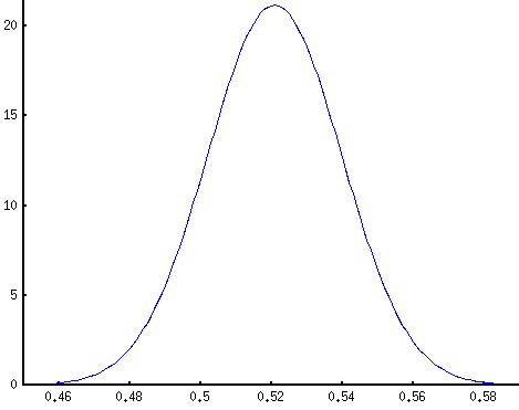
This is concentrated in a small region (note the x-axis) around 50 / (50 + 46) = 52.1%, Obama’s fraction of the two-way vote. The probability that Obama is ahead is the portion of mass to the right of pO’ = 50%:
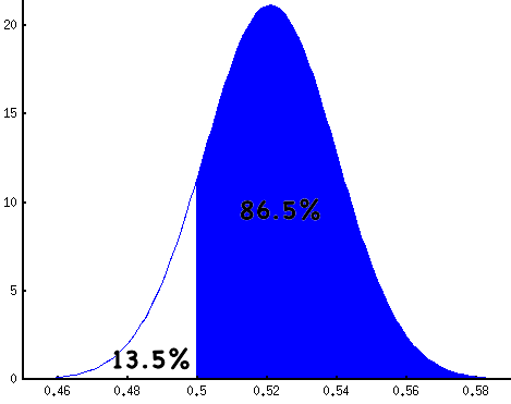
This fraction is calculated numerically using an integral. It’s an important enough quantity to have a name, but not important enough to have a short, catchy name. It’s the regularized incomplete beta function,
P(Obama ahead) = I0.5(b, a) = I0.5(732 * 0.46, 732 * 0.50)
It can be calculated using a program like Mathematica or Octave, or by using an online calculator.
Another way of formulating this is to ask, “what is the fraction Δ by which a candidate must lead in a poll to have a 95% chance of really being ahead?” For a small sample, Δ will be large. For a large sample it will be small.
In a survey of N voters, a candidate with a lead of Δ can claim his chance of leading is:
P(leading) = I0.5(N*(0.5-Δ), N*(0.5+Δ))
By inverting the regularized incomplete beta function, one can calculate what lead is necessary for 95% confidence. But that’s hard. Here’s a table to make things simpler:
| N | MoE | Δ | Δ/MoE |
|---|---|---|---|
| 100 | 10.0% | 16.36% | 1.6362 |
| 200 | 7.07% | 11.60% | 1.6402 |
| 500 | 4.47% | 7.35% | 1.6431 |
| 1000 | 3.16% | 5.20% | 1.6438 |
| 1500 | 2.58% | 4.25% | 1.6443 |
| 2000 | 2.24% | 3.68% | 1.6444 |
| 2500 | 2.00% | 3.29% | 1.6445 |
| 3000 | 1.83% | 3.00% | 1.6445 |
The ratio Δ/MoE; quickly approaches a constant, somewhere around 1.644. Hence the rule I mentioned at the beginning of the post. If a candidate is ahead by more than about 1.6 times the sampling error, that corresponds to 95% confidence. If the lead is equal to the sampling error, this corresponds to about 85% confidence. A lead of half the sampling error corresponds to about 70% confidence.
]]>But before checking out for a few months, I’ve got one last Presidential Primary post left in me.
The question for the last few weeks has been “why is Hillary still in this race?” She can’t win a majority of pledged delegates, overall delegates, states, or votes (unless you use very strange definitions of who “counts”). Could she have something up her sleeve with Michigan and Florida?
According to Daily Kos, here was the delegate count at the end of the night:
| Pledged | Super | Total | Needed | |
|---|---|---|---|---|
| Obama | 1,656.5 | 304.5 | 1,961 | 64 |
| Clinton | 1,501.5 | 277.5 | 1,779 | 246 |
| Remaining | 86 | 214 | 300 |
Obama passed 1,622 pledged delegates tonight and claimed a majority. But that excludes Florida and Michigan. Florida had 185 delegates and Michigan had 156. To get an absolute majority of pledged delegates including Florida and Michigan, he’d need 1,622 + (185 + 156)/2 = 1792.5 delegates. With only 86 pledged delegates left, there’s no way he can make Florida and Michigan irrelevant.
Or so goes the argument. But what did those excluded Florida and Michigan actually look like?
| Florida | Michigan | |
|---|---|---|
| Obama | 69 | 0 |
| Clinton | 105 | 73 |
| Uncommitted | 0 | 55 |
I don’t know precisely how the “Uncommitted” delegates work, but I imagine they’d be under enormous pressure to vote for Obama at the convention. Add those in and you get:
| Pledged | Fl.+Mi. | Total Pledged | Needed | |
|---|---|---|---|---|
| Obama | 1,656.5 | 124 | 1780.5 | 12 |
| Clinton | 1,501.5 | 178 | 1679.5 | 113 |
| Remaining | 86 | 0 | 86 |
So if you include the Florida and Michigan delegations, he hasn’t passed that magic mark, but he’s extremely close. And more interestingly, he’s the only one that can pass that mark. Hillary needs 113 pledged delegates for a majority, but there are only 86 left. This is because of the Edwards delegates.
If you don’t give Obama the 55 uncommitted delegates from Michigan though, he’s unlikely to pass the 50% mark, even by June 3. Could that be the trick? It seems a bit far-fetched. We’ll find out in three months when I start paying attention again!
]]>One thing that’s certain about Edwards’ decision is that it’s a good one for the Democratic party. Because each state awards delegates proportional to its popular vote, he could have grabbed maybe 5-10% of the delegates. This would have almost certainly prevented either Clinton or Obama from getting a majority, and led to a brokered convention. Now, that could only happen if there were an exceptionally close delegate race.
]]>At the same time, I know that the Hillary machine is trying to project a sense of inevitability. It’s all part of their plan, and I don’t want to buy into it.
A couple reactions to the article I linked to:
- Fish dismisses Obama as a VP candidate too quickly. So we’re ready for a black president, we’re ready for a woman president, but not both at the same time? I don’t buy it. No one’s accused Hillary of being charismatic, and a Hillary/Obama ticket could generate a lot of excitement to get out the vote.
- I suspect Fish’s pick is Bill Richardson. He’s been a governor (unlike Hillary) and Fish believes that he pulls a best of both worlds that Obama cannot: he’s a minority, but still looks white and has a white-sounding name. I’m still skeptical of all this talk that the voters will freak out if a ticket has no white male. But Fish’s other point about Richardson is excellent: his main problem now is that he has difficulty staying on message, and has delivered some really brain-dead responses to unexpected questions. I have great faith that the Hillary camp would whip him into shape.
I’m still rooting for Barack Obama to win the nomination, but if Hillary does win, I’d be happy with either of the pairings mentioned above.
]]>